Greater flexibility means more robustness
Going beyond the rather trivial result of the first proposition, the second proposition (see original post) was:
Greater flexibility means, for a given initial withdrawal rate, the portfolio is more robust against prematurely running out of money if that initial withdrawal was poorly chosen (added here) or returns were lower than found historically.
In the following analysis, robustness has been defined as where the portfolio has not prematurely become exhausted. However, this ignores what might be labelled ‘income robustness’ where by adopting flexibility, the portfolio income could fall below the minimum ‘core’ spending requirement. It is worth noting that where the portfolio runs out of money, income will have permanently fallen below that minimum.
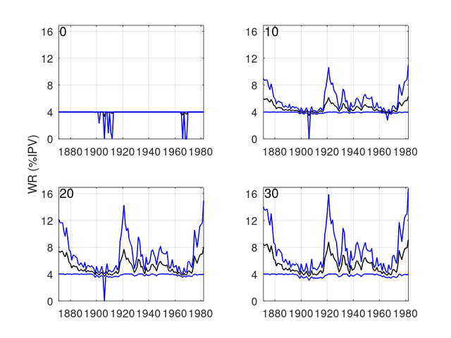
In the following figure, the mean (black line), minimum, and maximum real withdrawal rates have been plotted as a function of the starting year of each historical retirement for F=0 (i.e., constant dollar with no flexibility), F=10, F=20, and F=30 (the value of F is marked in the top left of each panel). It should also be remembered (as per my original post), I am using a 40 year retirement period and a 60/40 TSM/TBM portfolio (Simba data).
![Image]()
From the figure, the following points can be made:
1. The number of retirements where the minimum withdrawal fell to zero or close to zero, decreased as F was increased (for F=10 and F=20, this only occurred for the retirement that started in 1906 plotted in my earlier post, viewtopic.php?p=7818757#p7818757). While it is fairly well known in these parts, it is still worth noting that for F=0, the retirements where the withdrawal fell to zero (i.e., ‘failure’ in SWR terms) were clustered in retirements starting in the first decade of the 20th century and in the mid to late 1960s.
2. Increasing F increases the variability of withdrawals (e.g. as indicated by the difference between the maximum and minimum values).
3. For ‘good’ retirements, there was considerable upside in adopting even a relatively small amount of flexibility.
4. While it is not easy to see in the graphs, the mean withdrawal for F>0 tended to be higher than that for F=0 except for a handful of retirements (e.g., 1899), with the number increasing with increasing F.
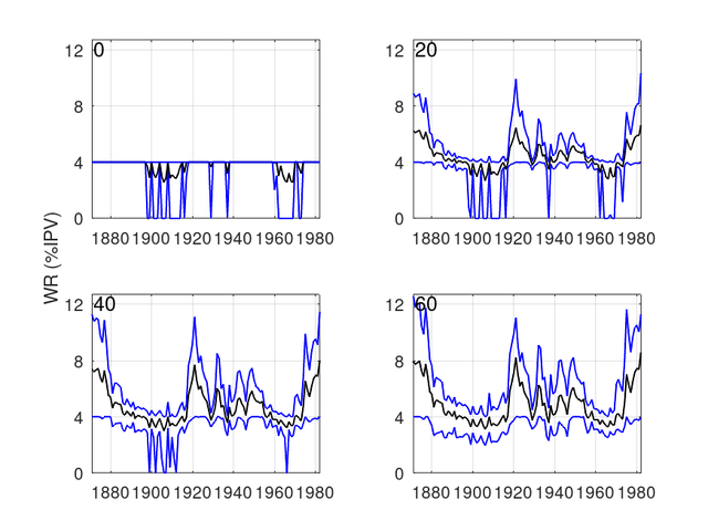
Now let’s repeat the analysis under harsher conditions using a reduction in historical real returns of 1 percentage point – this reduction could be because inflation was higher, nominal returns lower, or a combination of both. Since we are using historical data, the sequence of returns is left unaffected, but their values are changed. Note the different values of F (0, 20, 40, and 60) used in this graph.
![Image]()
Again, there are a few things to note:
1. The most obvious (and least surprising) of which is that worse conditions led to worse outcomes both in terms of the number of times the withdrawals fell to zero, but also the mean withdrawals.
2. Much greater flexibility (F=60) was required with worse conditions to avoid the withdrawals falling to zero.
3. On an optimistic note (if we can manage that here at Bogleheads!), even with these poor conditions, there were still plenty of retirements that provided income throughout the retirement period (with or without flexibility).
The minimum value of F (to the nearest 10) required to ensure that withdrawals did not fall to zero for different values of return reduction is given in the following table:
From the table, given an initial withdrawal of 4%, then greater flexibility was required for worse conditions in order to maintain a given level of robustness (in this case, zero cases of the income falling to zero).
cheers
StillGoing
Going beyond the rather trivial result of the first proposition, the second proposition (see original post) was:
Greater flexibility means, for a given initial withdrawal rate, the portfolio is more robust against prematurely running out of money if that initial withdrawal was poorly chosen (added here) or returns were lower than found historically.
In the following analysis, robustness has been defined as where the portfolio has not prematurely become exhausted. However, this ignores what might be labelled ‘income robustness’ where by adopting flexibility, the portfolio income could fall below the minimum ‘core’ spending requirement. It is worth noting that where the portfolio runs out of money, income will have permanently fallen below that minimum.
In the following figure, the mean (black line), minimum, and maximum real withdrawal rates have been plotted as a function of the starting year of each historical retirement for F=0 (i.e., constant dollar with no flexibility), F=10, F=20, and F=30 (the value of F is marked in the top left of each panel). It should also be remembered (as per my original post), I am using a 40 year retirement period and a 60/40 TSM/TBM portfolio (Simba data).

From the figure, the following points can be made:
1. The number of retirements where the minimum withdrawal fell to zero or close to zero, decreased as F was increased (for F=10 and F=20, this only occurred for the retirement that started in 1906 plotted in my earlier post, viewtopic.php?p=7818757#p7818757). While it is fairly well known in these parts, it is still worth noting that for F=0, the retirements where the withdrawal fell to zero (i.e., ‘failure’ in SWR terms) were clustered in retirements starting in the first decade of the 20th century and in the mid to late 1960s.
2. Increasing F increases the variability of withdrawals (e.g. as indicated by the difference between the maximum and minimum values).
3. For ‘good’ retirements, there was considerable upside in adopting even a relatively small amount of flexibility.
4. While it is not easy to see in the graphs, the mean withdrawal for F>0 tended to be higher than that for F=0 except for a handful of retirements (e.g., 1899), with the number increasing with increasing F.
Now let’s repeat the analysis under harsher conditions using a reduction in historical real returns of 1 percentage point – this reduction could be because inflation was higher, nominal returns lower, or a combination of both. Since we are using historical data, the sequence of returns is left unaffected, but their values are changed. Note the different values of F (0, 20, 40, and 60) used in this graph.

Again, there are a few things to note:
1. The most obvious (and least surprising) of which is that worse conditions led to worse outcomes both in terms of the number of times the withdrawals fell to zero, but also the mean withdrawals.
2. Much greater flexibility (F=60) was required with worse conditions to avoid the withdrawals falling to zero.
3. On an optimistic note (if we can manage that here at Bogleheads!), even with these poor conditions, there were still plenty of retirements that provided income throughout the retirement period (with or without flexibility).
The minimum value of F (to the nearest 10) required to ensure that withdrawals did not fall to zero for different values of return reduction is given in the following table:
Code:
Return Reduction (percentage points)0.00.51.01.52.02.53.0Min F30406060708080cheers
StillGoing
Statistics: Posted by StillGoing — Sun Apr 14, 2024 1:58 am — Replies 10 — Views 848